Choosing a Rocket Parachute: Why Descent Speed Matters

How big should a rocket’s parachute be? Most online calculators make this straightforward: enter the rocket’s recovery mass, choose a descent speed, and calculate a parachute diameter.

That is a useful starting point. If you accept 6 m/s—about 20 ft/s—as a suitable landing speed, the familiar mass-based calculation gives you a parachute size under its assumed drag conditions. But it leaves an important question unanswered: why is that speed suitable for your rocket?

Jump to the Chute Calculator..

Mass sets the load. Speed changes the landing.

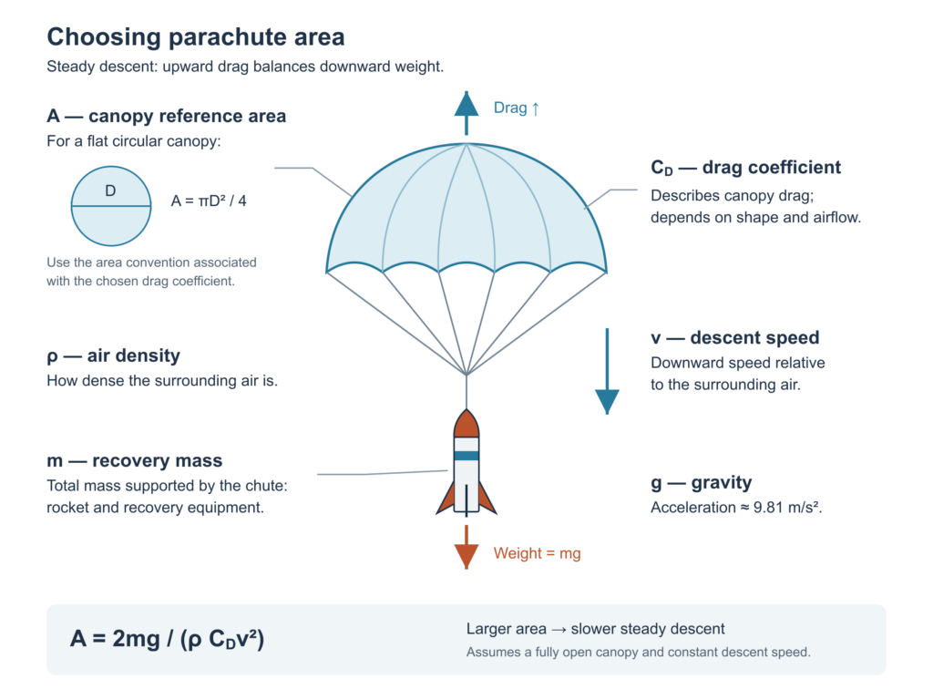
A parachute slows a rocket by producing drag. During steady descent, that drag balances the rocke’s weight. A heavier rocket needs more parachute area to maintain the same descent speed.

The usual relationship is:

\[
A=\frac{2mg}{\rho C_Dv^2}
\]

Here, (A) is parachute area, (m) is recovery mass, (g) is gravitational acceleration, ($\rho$) is air density, ($C_D$) describes the parachute’s drag, and (v) is the chosen descent speed.

Mass is usually known. The choice of speed deserves more attention: halving the descent speed requires four times the parachute area, assuming the same air density and drag coefficient. For a circular parachute, that means twice the diameter.
What happens when the rocket reaches the ground?

The rocket’s kinetic energy is:

\[
E_k=\frac12mv^2
\]

A small increase in speed can therefore make a substantial difference to the landing. The same rocket arriving at 6 m/s carries 44% more kinetic energy than it does at 5 m/s.

How abruptly that energy is removed matters too. A rocket stopping over a short distance experiences a greater average stopping force than one slowing over a longer distance. Grass, soil, the rocket’s orientation, and deformation all affect that distance. Five centimetres of grass does not necessarily provide five centimetres of cushioning.

The fins also matter a lot. Their thickness, root width, span, grain direction, and attachment affect their ability to withstand a landing load. Mass alone cannot tell us whether a particular landing speed is acceptable.
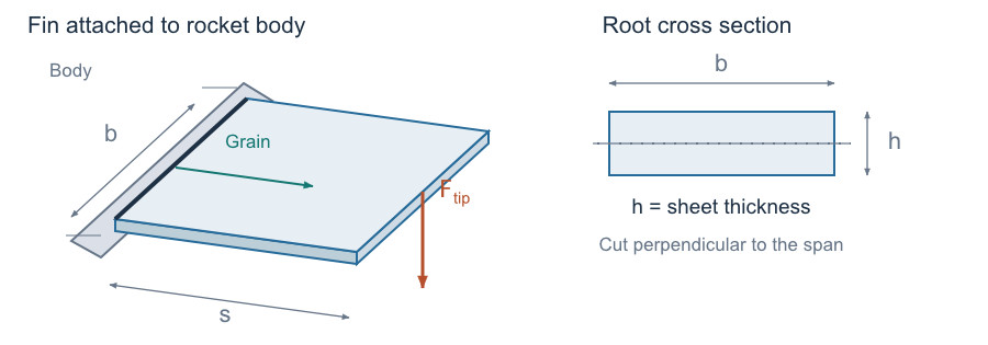
Fin dimensions and an applied force.

A simple model to make the choice more informed

To explore this, I modeled a balsa wood fin as a small cantilever beam: fixed at the rocket body, with a force acting perpendicular to the fin at its tip.

The analysis connects three estimates:

  1. The bending load the fin might withstand.
  2. The landing speed compatible with that load over an assumed stopping distance.
  3. The parachute area needed to achieve that speed.

For illustrative purposes, a 195 g rocket, with a 60 mm root chord, 60 mm span, and 3 mm thick balsa fins, the model gives a candidate descent speed of approximately 3.4 m/s when using a 50 mm stopping distance and no additional load allowance. With the same drag assumptions, that corresponds to a circular parachute approximately 26 inches in diameter, compared with about 15 inches at 6 m/s.

Those numbers are an example, not a proven safe limit. The calculation assumes sound balsa wood, favorable grain alignment, a secure attachment, and a particular distribution of force. A corner strike, twisting, or a shorter stopping distance could produce a more severe result.

The model’s value is that the assumptions are visible—and we can see how changing them changes the answer.

A larger parachute has a cost

Slower descent generally reduces landing loads, but it also means more time in the air and more opportunity to drift.

In a steady 3 m/s wind, descending through 100 metres takes about 17 seconds at 6 m/s, producing roughly 50 metres of drift. At 3.4 m/s, it takes about 29 seconds, producing roughly 88 metres of drift.

A smaller parachute gets the rocket down sooner, but may land it too hard. A larger parachute softens the landing while increasing the distance you might have to walk—or the chance of your rocket leaving the recovery field and into a tree!
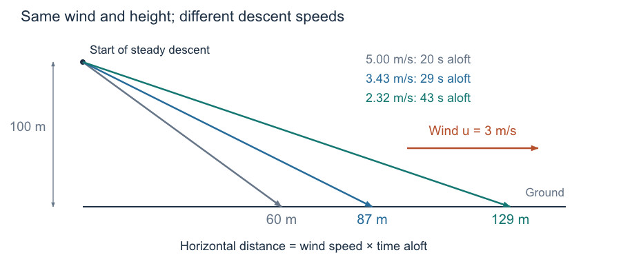
Faster and slower descents drifting in the same wind.

Choosing the Descent Velocity

A mass-based parachute calculator is useful when you already have a suitable target descent speed; OpenRocket or RockSim are super helpful in this regard. Understanding the landing helps you decide what that target should be.

The aim is to choose a speed that balances the rocket’s construction, the expected landing conditions, and the available recovery area. Even a simplified calculation can make that choice more informed, especially when followed by measured descent rates and observations from actual flights.

Before sizing the parachute, we need to estimate the landing speed the fins can tolerate. The following formula combines the fin dimensions, material bending strength, rocket recovery mass, and stopping distance to estimate a limiting descent velocity:

\[
\boxed{
v_*=
\sqrt{
\frac{2d}{m}
\left(
\frac{\sigma_{\mathrm{bend}},b,t^2}{6s}
-mg
\right)
}
}
\]

where:

  • ($v_*$) — estimated limiting descent velocity (m/s)
  • (d) — stopping distance during impact (m)
  • (m) — total descending mass, including recovery gear (kg)
  • ($\sigma_{\mathrm{bend}}$) — fin material bending strength (Pa)
  • (b) — fin root chord (m)
  • (t) — fin thickness (m)
  • (s) — fin span (m)
  • (g) — gravitational acceleration, approximately ($9.81\ \mathrm{m/s^2}$)

The term ($\sigma_{\mathrm{bend}}bt^2/(6s)$) estimates the bending load a single fin can withstand, treating it as a rectangular cantilever loaded at its tip across its thickness. The remaining expression comes from equating the rocket’s kinetic energy to the work done by the net stopping force over distance (d).

The resulting velocity can then be substituted into the parachute sizing formula. This simplified model assumes a constant stopping force and includes no safety margin, so the result represents an estimated limit rather than a guaranteed damage-free landing speed. The estimated bending load must exceed (mg) for a positive limiting velocity to exist which makes sense otherwise they couldn’t support the rocket even when sitting still on the ground.


The Interactive Parachute Sizing Calculator

Loading the parachute calculator. JavaScript must be enabled.


Want the full analysis?

Download the accompanying PDF for the beam-flexure derivation, worked examples, parachute geometry, and a closer look at the assumptions behind the estimates.

Rocket Engineering Enrichment Program

A Hands-On Rocket Engineering Experience

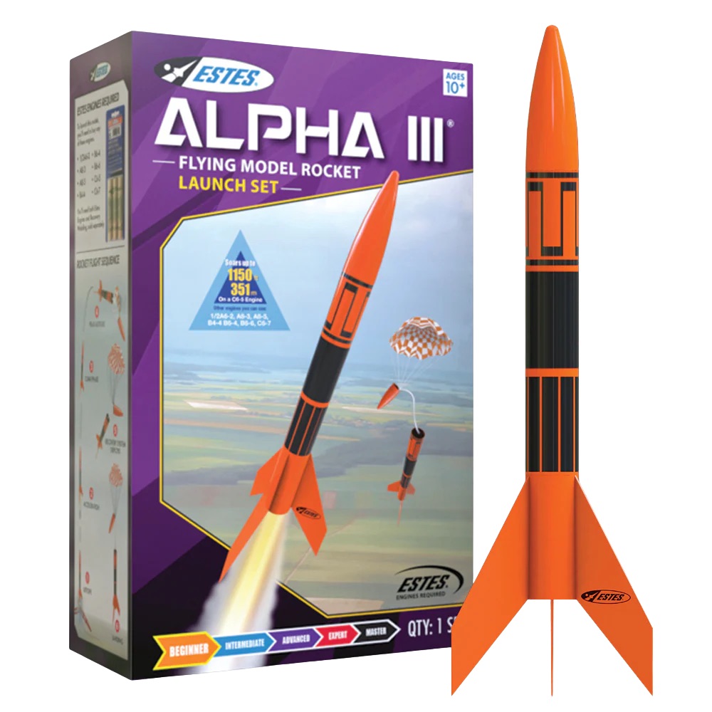
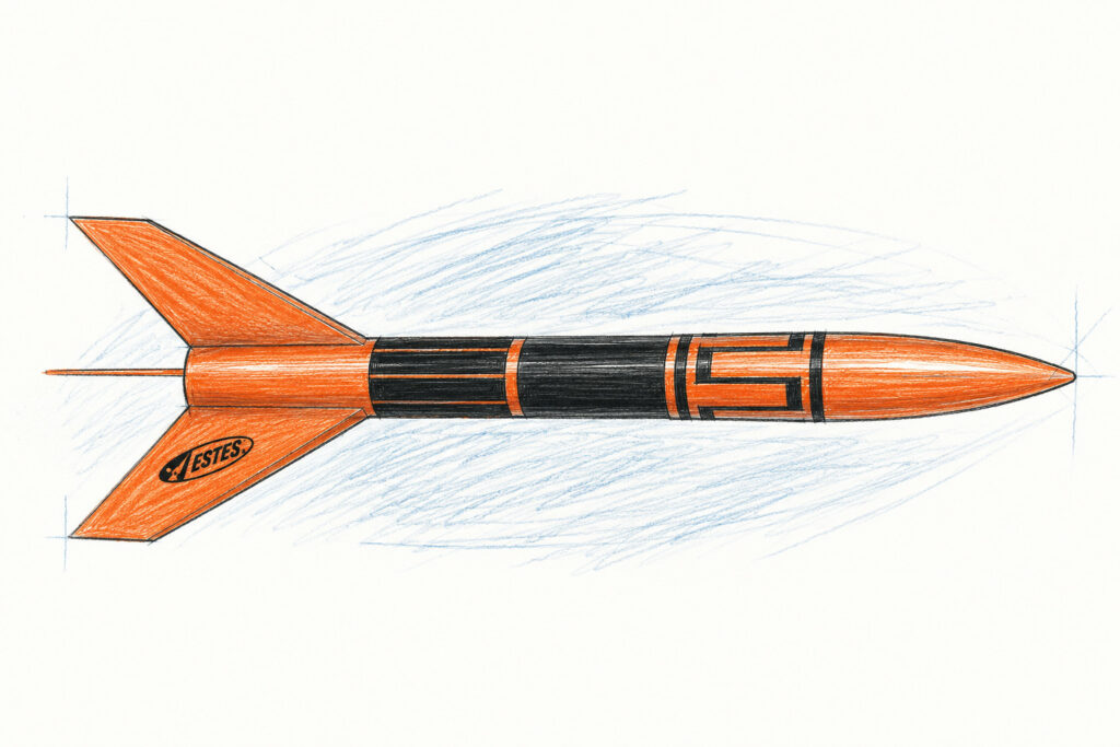
Estes Alpha III illustration

What happens when you combine engineering, physics, teamwork, and real rocket launches?

Students don’t just learn about rockets—they build one, launch it, analyze it, and discover the science that makes it fly.

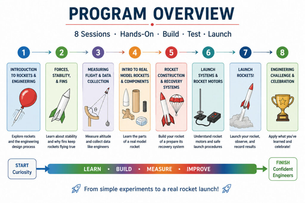
This enrichment program is a project-based introduction to aerospace engineering and scientific thinking. Through a series of engaging hands-on activities, students explore how real engineers design, test, and improve rockets while developing problem-solving skills that extend far beyond the launch field.


What Students Will Do

Throughout the program students will:

  • Build and personalize their own model rocket
  • Learn how rockets generate thrust
  • Explore Newton’s Laws of Motion through demonstrations and experiments
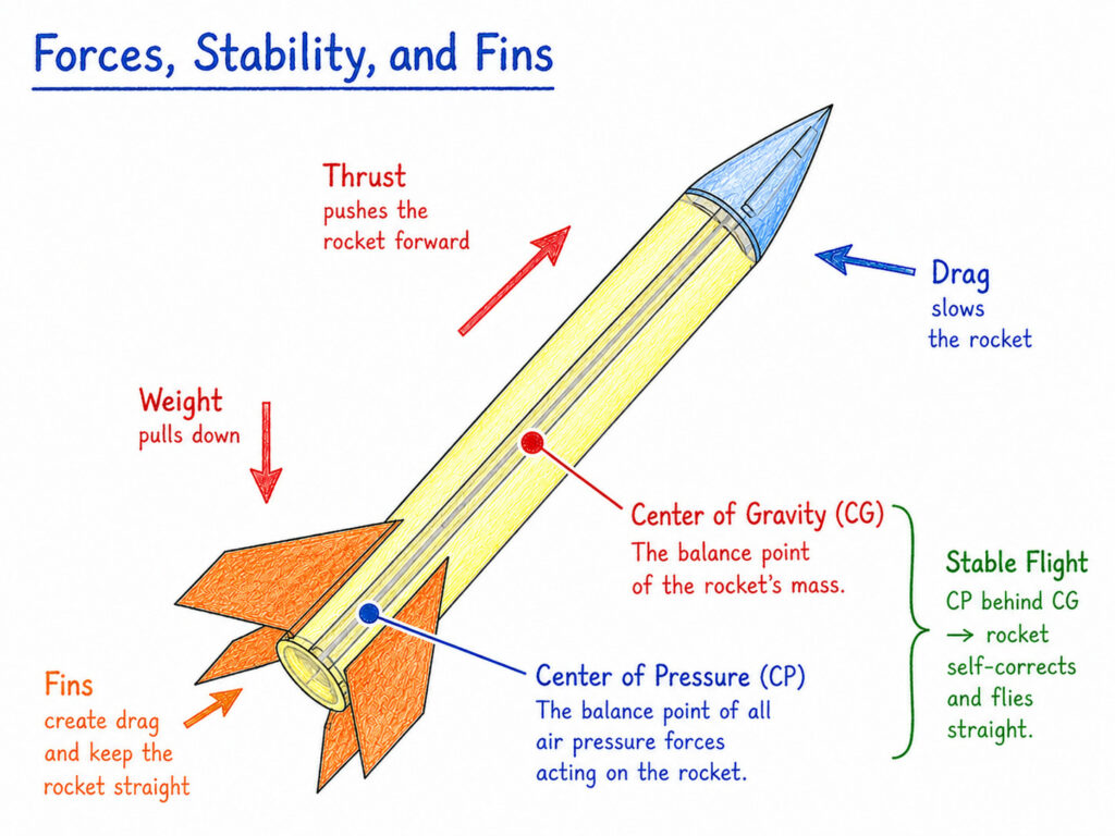
  • Discover how fins, mass, and balance affect stability
  • Measure rocket performance using real flight data
  • Practice engineering design through testing and redesign
  • Safely launch their own rocket
  • Take their completed rocket home
Build-Launch-Discover

Every lesson combines a short interactive presentation with hands-on activities that keep students actively engaged.


Rocket diagram labeled

Engineering Through Experience

Students experience the ideas firsthand.

Activities include:

  • Balloon rocket experiments
  • Paper rocket design challenges
  • Rocket stability investigations
  • Model rocket construction
  • Flight prediction and analysis
  • Real launch procedures
  • Engineering design challenges

Students are encouraged to ask questions, make predictions, test ideas, and improve their designs just as engineers do.


Program Overview flowchart

Safety Comes First

Safety first poster

Model rocketry has been enjoyed safely for decades when proper procedures are followed.

Students learn:

  • Launch range safety
  • Rocket inspection procedures
  • Safe motor installation
  • Launch pad operation
  • Countdown and launch protocols
  • Recovery procedures

Safety isn’t simply discussed—it becomes part of the engineering process through structured checklists and instructor supervision.


What Makes This Program Different?

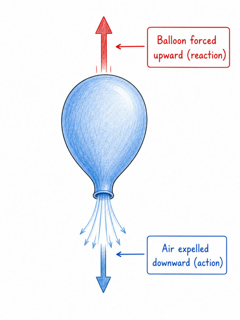
Newton's 3rd Law: Action-Reaction

Designed for curious minds. Whether a student dreams of becoming an engineer, loves building things, or simply enjoys discovering how the world works, this program provides an exciting introduction to STEM through one of the most inspiring engineering projects ever created—a flying rocket.

Every student leaves with new knowledge, greater confidence, practical engineering experience, and a rocket they built themselves. The program connects each activity into a complete engineering experience where students learn how scientific ideas explain what they observe.

Topics include:

  • Newton’s Laws of Motion
  • Thrust and propulsion
  • Aerodynamics
  • Stability and center of gravity
  • Drag and recovery systems
  • Measurement and data collection
  • Engineering design and iteration

Concepts are presented in an age-appropriate way, emphasizing curiosity and understanding rather than heavy mathematics.


Ready for Launch?

What’s Included

✓ Eight hands-on STEM sessions

✓ Alpha III model rocket kit

✓ Launch motor(s)

✓ All classroom materials

✓ Safety instruction

✓ Final launch event with experienced rocketeers

Interested in bringing Rocket Engineering to your school, homeschool group, or enrichment program?

Contact me for upcoming sessions, scheduling, and registration details.

The Tsiolkovsky Rocket Equation: From Conservation of Momentum to a Model Rocket

The Tsiolkovsky Rocket Equation is one of the most elegant results in classical mechanics. Despite describing everything from hobby rockets to missions leaving the Solar System, the underlying mathematics is surprisingly approachable. Starting with nothing more than conservation of momentum and a little calculus, we can derive an equation that predicts the maximum velocity change a rocket is capable of producing–often called “Delta-V”.

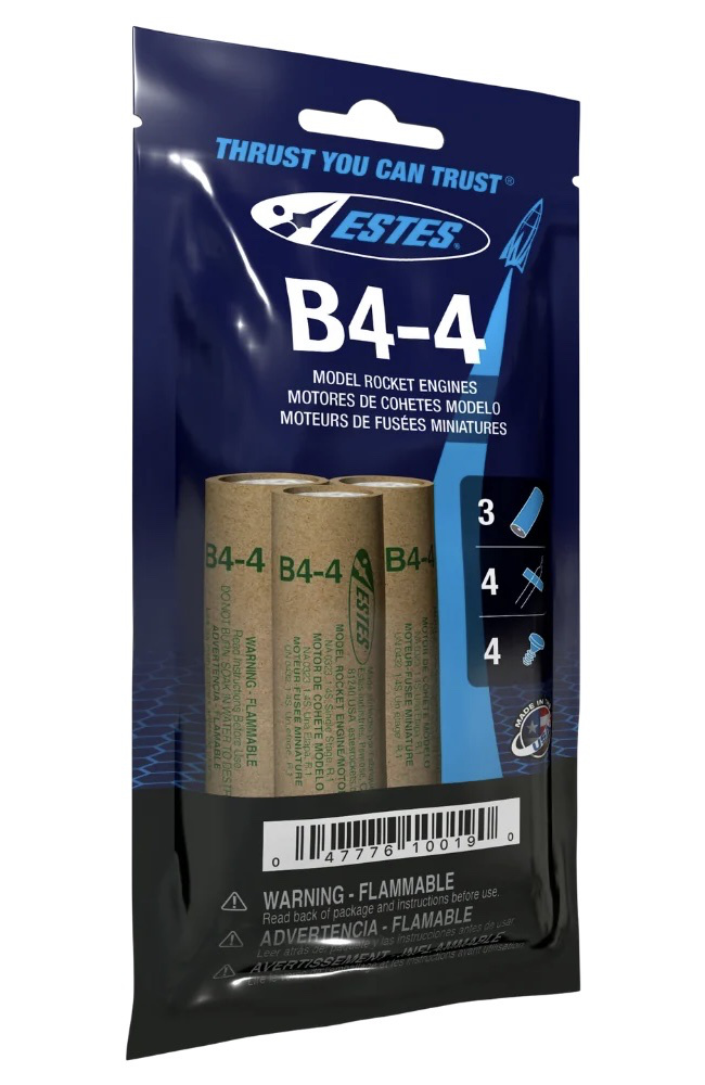
In this article we’ll derive the rocket equation from first principles and then apply it to a familiar model rocket—the Estes Alpha III powered by a B4-4 engine.


Why Rockets Are Different

Most vehicles push against something already present.

  • A car pushes against the road.
  • An airplane pushes against the air.
  • A boat pushes against the water.

A rocket is different because it carries its own reaction mass. High-speed exhaust gases are expelled from the nozzle, and by Newton’s Third Law the rocket is accelerated in the opposite direction.

A rocket becomes lighter as it accelerates because it is continuously throwing away part of its own mass (the fuel). That changing mass is exactly what makes rockets mathematically interesting.


Step 1 — Start with Conservation of Momentum

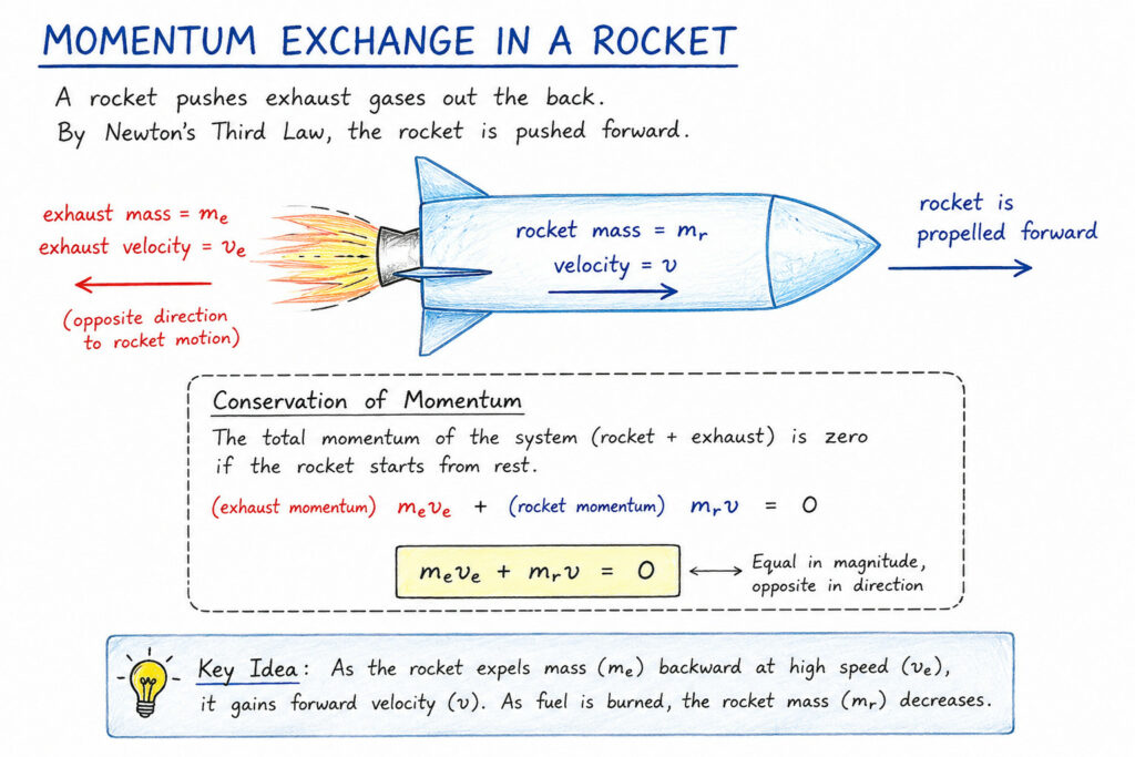
Illustration of Momentum Exchange in a Rocket

The total momentum of the rocket and the expelled exhaust must remain constant. Momentum is defined as

\[
p = mv
\]

If the rocket starts from rest, the momentum of the rocket must exactly balance the momentum carried away by the exhaust gases.

\[
m_{\text{fuel}} v_e + m_{\text{rocket}} v = 0
\]

or

\[
m_{\text{fuel}} v_e = -m_{\text{rocket}} v
\]

The negative sign simply reminds us that the rocket and exhaust travel in opposite directions.


Step 2 — Recognize that Mass is Changing

This equation is only true for an instant in time because things keep changing. As fuel burns,

  • total rocket mass decreases,
  • fuel mass decreases as it leaves the rocket as exhaust
  • rocket velocity increases.

Instead of dealing with finite changes, we examine an infinitesimally small amount of fuel leaving the rocket.

This gives

\[
dm \, v_e = – M_r \, dv
\]

where

  • \(dm\) is a tiny amount of fuel expelled,
  • \(v_e\) is the exhaust velocity
  • \(M_r\) is the instantaneous rocket mass,
  • \(dv\) is the tiny increase in rocket velocity.

Step 3 — Separate the Variables

Rearranging to solve for the rocket’s velocity \(dv\) gives

\[
\frac{v_e}{M_r} \, dm = – dv
\]

or

\[
dv = – v_e \frac{dm}{M_r}
\]

Now the rocket’s changing velocity (\(dv\)) is one side and the changing fuel mass (\(dm\)) is on the other. This form is ready for integration.


Step 4 — Integrate During the Entire Burn

Assuming the exhaust velocity remains approximately constant during the burn,

\[
\int_{v_0}^{v_f} dv =
– v_e \, \int_{M_0}^{M_f}
\frac{1}{M_r} \, dm
\]

The left side is straightforward,

\[
v_f \, – \, v_0 = \Delta v
\]

while the right side becomes the natural logarithm,

\[
-v_e \left[\ln M_f \, – \, \ln M_0\right]
\]

Using logarithm identities,

\[
\boxed{\Delta v = v_e
\ln\left(\frac{M_0}{M_f}\right)}
\]

This is the famous Tsiolkovsky Rocket Equation.


Applying the Equation to an Estes Alpha III

Now let’s see how well this ideal equation predicts the performance of a real model rocket. For this example we’ll use the specifications provided on the Estes website:

Estes Alpha III

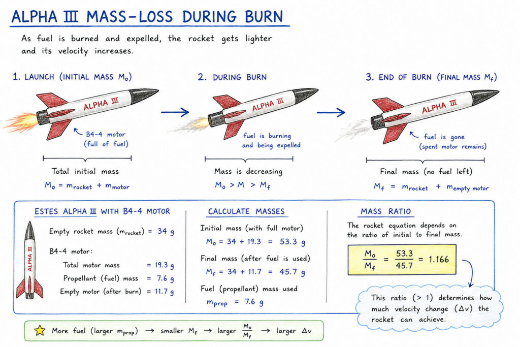
  • Empty rocket mass: 34.0 g

Estes B4-4 Motor

  • Motor mass: 19.3 g
  • Propellant mass: 7.6 g
  • Total impulse: 5.0 N·s
  • Burn time: 1.10 s

The rocket begins flight carrying the full motor. Therefore

\[
M_0 = 34.0 + 19.3 = 53.3\text{ g}
\]

After the propellant is burned,

\[
M_f = 53.3 \, – \, 7.6 = 45.7\text{ g}
\]

The mass ratio is therefore

\[
\frac{M_0}{M_f} = 1.166
\]

Taking the natural logarithm,

\[
\ln(1.166) = 0.154
\]

The remaining unknown is the effective exhaust velocity, \(v_e\). One estimate comes from the motor’s total impulse, which is provided in the motor’s specification sheet.

Impulse is the total push delivered by a force over time:

\[
I = F_{\text{avg}} \cdot \Delta t
\]

Impulse is also equal to a change in momentum:

\[
I = \Delta p
\]

Since momentum is

\[
p = mv
\]

the motor’s impulse can be interpreted as the momentum carried away by the expelled propellant. If the propellant mass is \(m_p\) and the effective exhaust velocity is \(v_e\), then

\[
I \approx m_p v_e
\]

This is an idealized estimate, but it gives us a useful value for the rocket equation.

For the B4-4 motor:

\[
I = 5.0 \, \text{N} \cdot \text{s}
\\
m_p = 0.0076 \, \text{kg}
\]

Solving for effective exhaust velocity:

\[
v_e = \frac{I}{m_p}
\]

\[
v_e = \frac{5.0}{0.0076}
\approx 658 \, \text{m/s}
\]

Now substitute this into the rocket equation:

\[
\boxed{\Delta v = v_e
\ln\left(\frac{M_0}{M_f}\right)}
\]

Using the previously calculated mass ratio,

\[
\ln\left(\frac{M_0}{M_f}\right) = \ln(1.166) \approx 0.154
\]

Therefore,

\[
\Delta v = (658)(0.154)
\approx 101 \, \text{m/s}
\]

The ideal rocket equation predicts a maximum velocity change of approximately

\[
\boxed{\Delta v \approx 100 \, \text{m/s}}
\]

or about

\[
\boxed{225 \, \text{mph}}
\]


Alpha III mass loss diagram

Why Doesn’t the Rocket Reach This Speed?

If you’ve ever watched an Alpha III launch, you may notice that measured peak velocities are usually lower than this calculation predicts.

That’s because the Tsiolkovsky Rocket Equation is an ideal model.

It assumes:

  • no aerodynamic drag,
  • no gravity losses during powered flight,
  • perfectly constant exhaust velocity,
  • no energy lost to heating or turbulence.

A real rocket experiences all of these effects simultaneously.

Computer flight simulators such as OpenRocket include drag, changing thrust curves, atmospheric density, gravity, and coast phase dynamics, producing much more realistic predictions.

The rocket equation, however, still serves as the fundamental theoretical limit on rocket performance.


Final Thoughts

One of the remarkable aspects of the rocket equation is that it emerges from only two ideas:

  • Newton’s Third Law
  • Conservation of Momentum

Everything else follows naturally from calculus.

Although hobby rockets are tiny compared to launch vehicles carrying satellites or astronauts, they obey exactly the same physics. Whether launching an Estes Alpha III from a school field or sending a spacecraft toward Mars, every rocket ultimately answers to the same elegant equation first derived by Konstantin Tsiolkovsky over a century ago.