The Tsiolkovsky Rocket Equation: From Conservation of Momentum to a Model Rocket

The Tsiolkovsky Rocket Equation is one of the most elegant results in classical mechanics. Despite describing everything from hobby rockets to missions leaving the Solar System, the underlying mathematics is surprisingly approachable. Starting with nothing more than conservation of momentum and a little calculus, we can derive an equation that predicts the maximum velocity change a rocket is capable of producing–often called “Delta-V”.

In this article we’ll derive the rocket equation from first principles and then apply it to a familiar model rocket—the Estes Alpha III powered by a B4-4 engine.


Why Rockets Are Different

Most vehicles push against something already present.

  • A car pushes against the road.
  • An airplane pushes against the air.
  • A boat pushes against the water.

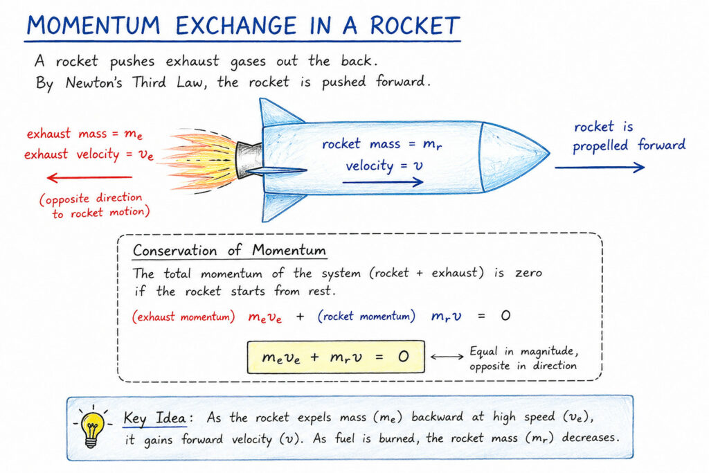
A rocket is different because it carries its own reaction mass. High-speed exhaust gases are expelled from the nozzle, and by Newton’s Third Law the rocket is accelerated in the opposite direction.

A rocket becomes lighter as it accelerates because it is continuously throwing away part of its own mass (the fuel). That changing mass is exactly what makes rockets mathematically interesting.


Step 1 — Start with Conservation of Momentum

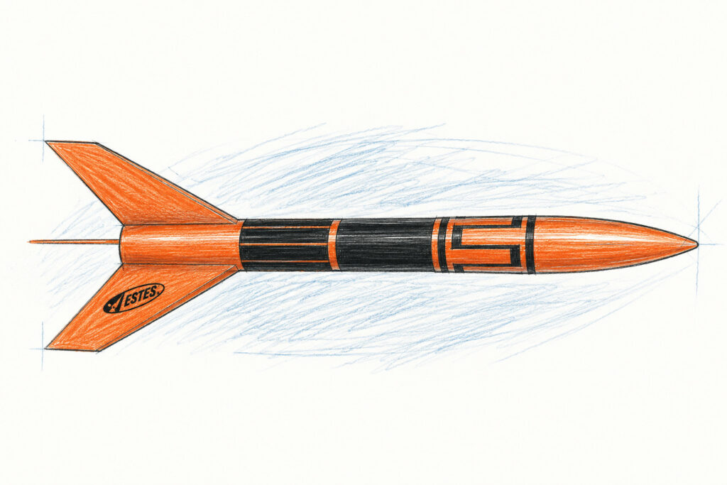
Illustration of Momentum Exchange in a Rocket

The total momentum of the rocket and the expelled exhaust must remain constant. Momentum is defined as

\[
p = mv
\]

If the rocket starts from rest, the momentum of the rocket must exactly balance the momentum carried away by the exhaust gases.

\[
m_{\text{fuel}} v_e + m_{\text{rocket}} v = 0
\]

or

\[
m_{\text{fuel}} v_e = -m_{\text{rocket}} v
\]

The negative sign simply reminds us that the rocket and exhaust travel in opposite directions.


Step 2 — Recognize that Mass is Changing

This equation is only true for an instant in time because things keep changing. As fuel burns,

  • total rocket mass decreases,
  • fuel mass decreases as it leaves the rocket as exhaust
  • rocket velocity increases.

Instead of dealing with finite changes, we examine an infinitesimally small amount of fuel leaving the rocket.

This gives

\[
dm \, v_e = – M_r \, dv
\]

where

  • \(dm\) is a tiny amount of fuel expelled,
  • \(v_e\) is the exhaust velocity
  • \(M_r\) is the instantaneous rocket mass,
  • \(dv\) is the tiny increase in rocket velocity.

Step 3 — Separate the Variables

Rearranging to solve for the rocket’s velocity \(dv\) gives

\[
\frac{v_e}{M_r} \, dm = – dv
\]

or

\[
dv = – v_e \frac{dm}{M_r}
\]

Now the rocket’s changing velocity (\(dv\)) is one side and the changing fuel mass (\(dm\)) is on the other. This form is ready for integration.


Step 4 — Integrate During the Entire Burn

Assuming the exhaust velocity remains approximately constant during the burn,

\[
\int_{v_0}^{v_f} dv =
– v_e \, \int_{M_0}^{M_f}
\frac{1}{M_r} \, dm
\]

The left side is straightforward,

\[
v_f \, – \, v_0 = \Delta v
\]

while the right side becomes the natural logarithm,

\[
-v_e \left[\ln M_f \, – \, \ln M_0\right]
\]

Using logarithm identities,

\[
\boxed{\Delta v = v_e
\ln\left(\frac{M_0}{M_f}\right)}
\]

This is the famous Tsiolkovsky Rocket Equation.


Applying the Equation to an Estes Alpha III

Now let’s see how well this ideal equation predicts the performance of a real model rocket. For this example we’ll use the specifications provided on the Estes website:

Estes Alpha III

  • Empty rocket mass: 34.0 g

Estes B4-4 Motor

  • Motor mass: 19.3 g
  • Propellant mass: 7.6 g
  • Total impulse: 5.0 N·s
  • Burn time: 1.10 s

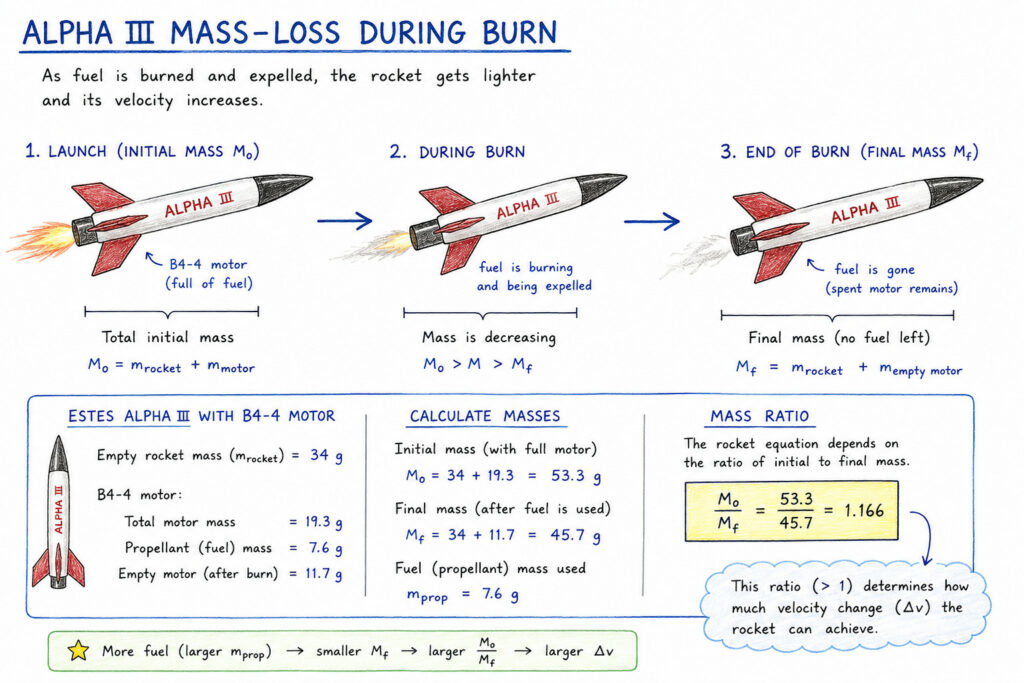
The rocket begins flight carrying the full motor. Therefore

\[
M_0 = 34.0 + 19.3 = 53.3\text{ g}
\]

After the propellant is burned,

\[
M_f = 53.3 \, – \, 7.6 = 45.7\text{ g}
\]

The mass ratio is therefore

\[
\frac{M_0}{M_f} = 1.166
\]

Taking the natural logarithm,

\[
\ln(1.166) = 0.154
\]

The remaining unknown is the effective exhaust velocity, \(v_e\). One estimate comes from the motor’s total impulse, which is provided in the motor’s specification sheet.

Impulse is the total push delivered by a force over time:

\[
I = F_{\text{avg}} \cdot \Delta t
\]

Impulse is also equal to a change in momentum:

\[
I = \Delta p
\]

Since momentum is

\[
p = mv
\]

the motor’s impulse can be interpreted as the momentum carried away by the expelled propellant. If the propellant mass is \(m_p\) and the effective exhaust velocity is \(v_e\), then

\[
I \approx m_p v_e
\]

This is an idealized estimate, but it gives us a useful value for the rocket equation.

For the B4-4 motor:

\[
I = 5.0 \, \text{N} \cdot \text{s}
\\
m_p = 0.0076 \, \text{kg}
\]

Solving for effective exhaust velocity:

\[
v_e = \frac{I}{m_p}
\]

\[
v_e = \frac{5.0}{0.0076}
\approx 658 \, \text{m/s}
\]

Now substitute this into the rocket equation:

\[
\boxed{\Delta v = v_e
\ln\left(\frac{M_0}{M_f}\right)}
\]

Using the previously calculated mass ratio,

\[
\ln\left(\frac{M_0}{M_f}\right) = \ln(1.166) \approx 0.154
\]

Therefore,

\[
\Delta v = (658)(0.154)
\approx 101 \, \text{m/s}
\]

The ideal rocket equation predicts a maximum velocity change of approximately

\[
\boxed{\Delta v \approx 100 \, \text{m/s}}
\]

or about

\[
\boxed{225 \, \text{mph}}
\]


Alpha III mass loss diagram

Why Doesn’t the Rocket Reach This Speed?

If you’ve ever watched an Alpha III launch, you may notice that measured peak velocities are usually lower than this calculation predicts.

That’s because the Tsiolkovsky Rocket Equation is an ideal model.

It assumes:

  • no aerodynamic drag,
  • no gravity losses during powered flight,
  • perfectly constant exhaust velocity,
  • no energy lost to heating or turbulence.

A real rocket experiences all of these effects simultaneously.

Computer flight simulators such as OpenRocket include drag, changing thrust curves, atmospheric density, gravity, and coast phase dynamics, producing much more realistic predictions.

The rocket equation, however, still serves as the fundamental theoretical limit on rocket performance.


Final Thoughts

One of the remarkable aspects of the rocket equation is that it emerges from only two ideas:

  • Newton’s Third Law
  • Conservation of Momentum

Everything else follows naturally from calculus.

Although hobby rockets are tiny compared to launch vehicles carrying satellites or astronauts, they obey exactly the same physics. Whether launching an Estes Alpha III from a school field or sending a spacecraft toward Mars, every rocket ultimately answers to the same elegant equation first derived by Konstantin Tsiolkovsky over a century ago.

Revisiting Eddington: Measuring Starlight Deflection

In 1919, Arthur S. EddingtonFrank W. Dyson, and Mr. C. Davidson famously led an expedition to photograph a total solar eclipse and confirm Einstein’s prediction that massive bodies like the Sun could bend starlight. That photographic evidence became one of the first major tests of General Relativity. Here, using a digital remaster of the image, I’ll attempt to recreate the experiment measurements.

Tools and Data

These are the things needed to get going:

  • high-quality digitized image of the 1919 eclipse from ESO (link). This version uses image processing techniques to improve the image quality from the original photo plates.
  • sky map from Stellarium, set to the same region of sky but offset by 6 months to avoid the Sun’s interference.
  • Affinity Photo for image overlay and alignment.
  • Manual centroiding and pixel measurements to detect deflection.

Image Alignment

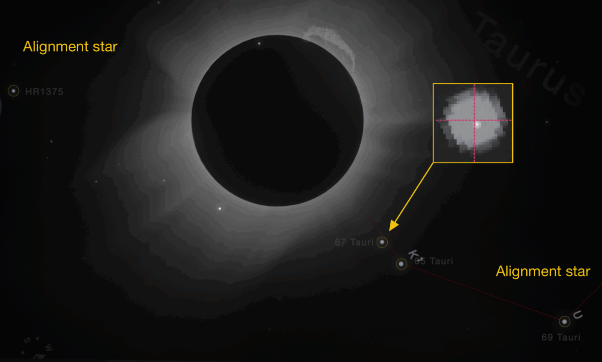
To ensure accuracy, I anchored both images using two distant reference stars — HR 1375 and 69 Tauri that are far enough from the eclipsed Sun to remain unaffected by gravitational lensing.

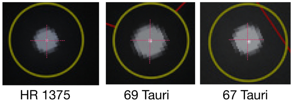
I loaded the original eclipse image as the background layer in Affinity Photo and locked it in place. Then I added the Stellarium-generated star field as a transparent overlay on top. By adjusting the opacity, I was able to see both sets of stars simultaneously for alignment. Notably, the star images from Stellarium appear significantly larger than the more compact and sharper ESO eclipse stars. In the cutouts shown in Figure 1, you can clearly see the difference. Each Stellarium star forms a large diffuse blob and the ESO image has its star as a bright point at the center.

After carefully stretching, rotating, and nudging the top layer, I aligned the two images so that the reference stars matched. It took a fair bit of trial and error, but I eventually achieved alignment within ±0.5 pixel, which is pretty decent for a manual process. This gave me confidence that any measured offsets for stars near the Sun were not due to alignment error — a point further supported by the zoomed-in cutouts shown in Figure 1, where the distant stars remain well-aligned.

Figure 1: Zoomed-in cutouts of reference and target stars. HR 1375 and 69 Tauri were used to align the two image layers within ±0.5 pixel. 67 Tauri shows a slight offset down and to the right, approximately 0.5-1.0 pixels — consistent with gravitational deflection predicted by General Relativity.

Here’s the annotated overlay, with 67 Tauri circled, and a zoomed inset revealing a small but visible offset between the eclipse photo and the reference sky.

potw1926a with Stellurium overlay annotated

Measuring the Deflection

The distance between 65 Tauri and 67 Tauri in the eclipse photo was measured as:

  • 158.7 pixels — determined by measuring the horizontal and vertical offsets between the two stars and applying Pythagoras’ theorem: \( \sqrt{105^2 + 119^2} \approx 158.7\)
  • Calculated angular separation340 arcseconds

This gives a plate scale of

Scale = 340 arcsec / 158.7 pixels ≈ 2.14 arcsec/pixel

Zooming in on 67 Tauri, the observed centroid deflection between the reference and eclipse position is down and right and approximately:

[0.75 to 1 pixels] × 2.14 arcsec/pixel ≈ 1.61 to 2.14 arcseconds

Comparison to Einstein’s Prediction

\( \delta = \frac{4GM}{c^2 R} \)

This is Einstein’s formula for the deflection angle ( \( \delta \) ) of starlight grazing the Sun, where:

Gravitational constant: \( G = 6.674 \times 10^{-11}~\text{m}^3\,\text{kg}^{-1}\,\text{s}^{-2} \\ \)
Mass of the Sun: \( M = 1.989 \times 10^{30}~\text{kg} \\ \)
Speed of light: \( c = 3.00 \times 10^8~\text{m/s}\\ \)
R is the radius/distance from the Sun’s center where the light ray is passing

At the solar limb where R is the same as the Sun’s radius then:

\( R = R_\odot = 6.96 \times 10^8~\text{m} \). Substitute this into the formula like so:

\( \delta = \frac{4GM}{c^2 R_\odot}
= \frac{4 \times (6.674 \times 10^{-11}) \times (1.989 \times 10^{30})}
{(3.00 \times 10^8)^2 \times (6.96 \times 10^8)} \)

\( \delta \approx 8.487 \times 10^{-6} \text{ radians} \), the deflection angle at the Sun’s rim.

And converting radians arcseconds (206265 arcseconds per radian) we get

\( \delta \approx 8.487 \times 10^{-6} \times 206265 \approx 1.75 \) arcseconds

Adjust for 67 Tauri’s apparent distance from the Sun

For 67 Tauri, which lies approximately 1.2–1.5 solar radii (r) from the Sun’s center, the expected deflection is:

\( \delta = \frac{4GM}{c^2 R_\odot} \cdot \frac{R_\odot}{r} \approx \frac{1.75^{”}}{r} \)

\( \delta \approx 1.17^{”} \quad \text{to} \quad 1.46^{”} \)

So, the measured deflection of approximately 1.61 to 2.14 arcseconds is a bit higher than expected. However, given error sources like:

  • Image projection distortions
  • Inaccuracies in the Stellarium overlay projection
  • Sub-pixel centroiding uncertainty
  • Manual centroiding for alignment and offset detection

…the result is remarkably close and very much in the spirit of Eddington’s original work.

This small experiment was a fun way to relive one of the greatest moments in science. With a bit of patience and publicly available images, it’s possible to experience Eddington’s achievement for yourself.


Angular Separation Calculation

To calculate the angular separation between 65 Tauri and 67 Tauri, use coordinates:

65 Tauri
RA = 04ʰ 25ᵐ 22.1655ˢ = 66.34235°
Dec = +22° 17′ 37.9375″ = +22.29387°

67 Tauri
RA = 04ʰ 25ᵐ 25.0152ˢ = 66.35423°
Dec = +22° 11′ 59.9876″ = +22.19999°

The spherical angular separation formula:

\(\theta = \arccos\left[
\sin(\delta_1)\sin(\delta_2) +
\cos(\delta_1)\cos(\delta_2)\cos(\alpha_1 – \alpha_2)
\right]\)

Substituting the values (converted to radians):

\(\alpha_1 = 1.157892441 \, \text{rad}, \quad \alpha_2 = 1.158099786 \, \text{rad}\)

\(\delta_1 = 0.3891014345 \, \text{rad}, \quad \delta_2 = 0.3874629194 \, \text{rad}\)

\(\theta = \arccos\left[\sin(0.38910..)\sin(0.38746..) + \cos(0.38910..)\cos(0.38746..)\cos(1.15789.. – 1.15809..) \right]\)

\(\theta \approx \arccos(0.9999986392) \approx 0.001649 \, \text{rad}\)

Converting to arcseconds:

\(\theta = 0.0016497 \times \frac{180 \times 3600}{\pi} \approx 340\)

So, the angular separation between 65 Tauri and 67 Tauri is approximately \( \boxed{340~\text{arcseconds}}\).